Deep neural networks and deep learning have become popular in past few years, thanks to the breakthroughs in research, starting from AlexNet, VGG, GoogleNet, and ResNet. In 2015, with ResNet, the performance of large-scale image recognition saw a huge improvement in accuracy and helped increase the popularity of deep neural networks.
This article discusses using a basic deep neural network to solve an image recognition problem. Here, emphasis is more on the overall technique and use of a library than perfecting the model. Part 2 explains how to improve the results.
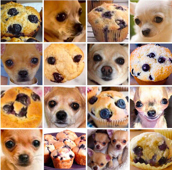
I wanted to use a deep neural network to solve something other than a “hello world” version of image recognition — MNIST handwritten letter recognition, for example. After going through the first tutorial on the TensorFlow and Keras libraries, I began with the challenge of classifying whether a given image is a chihuahua (a dog breed) or a muffin from a set of images that look similar.
The data set included with this article is formed by combining this source and searching the internet and applying some basic image processing techniques. The images in this data set are collected, used, and provided under the Creative commons fair usage policy. The intended use is (for scientific research in image recognition using artificial neural networks) by using the TensorFlow and Keras library. This solution applies the same techniques as given in https://www.tensorflow.org/tutorials/keras/classification.
Basically, there are no prerequisites to this article, but if you want to follow the code, it’s helpful to have basic knowledge of Python, numpy, and going through th eTensorFlow and Keras library.
Import the data
Clone the Git repository
$ git clone https://github.com/ScrapCodes/image-recognition-tensorflow.git
$ cd image-recognition-tensorflow
$ python
>>>
Import TensorFlow, Keras, and other helper libraries
I used TensorFlow and Keras for running the machine learning and the Pillow Python library for image processing.
Using pip, these can be installed on macOS as follows:
sudo pip install tensorflow matplotlib pillow
Note: Whether the use of sudo is required depends on how Python and pip is installed on your system. Systems configured with a virtual environment might not need sudo.
Importing the Python libraries.
# TensorFlow and tf.keras
import tensorflow as tf
from tensorflow import keras

# Helper libraries
import numpy as np
import matplotlib.pyplot as plt
import glob, os
import re

# Pillow
import PIL
from PIL import Image
Load the data
A Python function to preprocess input images. For images to be converted into numpy arrays, they must have same dimensions:
# Use Pillow library to convert an input jpeg to a 8 bit grey scale image array for processing.
def jpeg_to_8_bit_greyscale(path, maxsize):
        img = Image.open(path).convert('L')   # convert image to 8-bit grayscale
        # Make aspect ratio as 1:1, by applying image crop.
    # Please note, croping works for this data set, but in general one
    # needs to locate the subject and then crop or scale accordingly.
        WIDTH, HEIGHT = img.size
        if WIDTH != HEIGHT:
                m_min_d = min(WIDTH, HEIGHT)
                img = img.crop((0, 0, m_min_d, m_min_d))
        # Scale the image to the requested maxsize by Anti-alias sampling.
        img.thumbnail(maxsize, PIL.Image.ANTIALIAS)
        return np.asarray(img)
A Python function to load the data set from images, into numpy arrays:
def load_image_dataset(path_dir, maxsize):
        images = []
        labels = []
        os.chdir(path_dir)
        for file in glob.glob("*.jpg"):
                img = jpeg_to_8_bit_greyscale(file, maxsize)
                if re.match('chihuahua.*', file):
                        images.append(img)
                        labels.append(0)
                elif re.match('muffin.*', file):
                        images.append(img)
                        labels.append(1)
        return (np.asarray(images), np.asarray(labels))
We should scale the images to some standard size smaller than actual image resolution. These images are more than 170×170, so we scale them all to 100×100 for further processing:
maxsize = 100, 100
To load the data, let’s execute the following functions and load training and test data sets:
(train_images, train_labels) = load_image_dataset('/Users/yourself/image-recognition-tensorflow/chihuahua-muffin', maxsize)

(test_images, test_labels) = load_image_dataset('/Users/yourself/image-recognition-tensorflow/chihuahua-muffin/test_set', maxsize)
- train_images and train_lables is training data set.
- test_images and test_labels is testing data set for validating the model’s performance against unseen data.
Finally, we define the class names for our data set. Because this data has only two classes (an image can either be a Chihuahua or a Muffin), we have class_names as follows:
class_names = ['chihuahua', 'muffin']
Explore the data
In this data set, we have 26 training examples, of both Chihuahua and muffin images:
train_images.shape
(26, 100, 100)
Each image has its respective label – either a 0 or 1. A 0indicates a class_names[0] i.e. a chihuahua and 1 indicates class_names[1] i.e. a muffin:
print(train_labels)
[0 0 0 0 1 1 1 1 1 0 1 0 0 1 1 0 0 1 1 0 1 1 0 1 0 0]
For test set, we have 14 examples, seven for each class:
test_images.shape
(14, 100, 100)
print(test_labels)
[0 0 0 0 0 0 0 1 1 1 1 1 1 1]
Visualize the data set
Using the matplotlib.pyplot Python library, we can visualize our data. Make sure you have the matplotlib library installed.
Following Python helper function helps us draw these images on our screen:
def display_images(images, labels):
        plt.figure(figsize=(10,10))
        grid_size = min(25, len(images))
        for i in range(grid_size):
                plt.subplot(5, 5, i+1)
                plt.xticks([])
                plt.yticks([])
                plt.grid(False)
                plt.imshow(images[i], cmap=plt.cm.binary)
                plt.xlabel(class_names[labels[i]])
Let’s visualize the training data set, as follows:
display_images(train_images, train_labels)
plt.show()
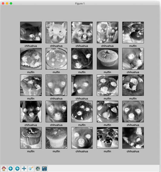
Note: The images are grayscaled and cropped in the preprocessing step of our images at the time of loading.
Similarly, we can visualize our test data set. Both training and test sets are fairly limited, so feel free to use Google search and add more examples and see how things improve or perform.
Preprocess the data
Scaling the images to values between 0 and 1
train_images = train_images / 255.0
test_images = test_images / 255.0
Build the model
Set up the layers
We have used four layers total. The first layer is to simply flatten the data set into a single array and does not get training. The other three layers are dense and use sigmoid as activation function:
# Setting up the layers.

model = keras.Sequential([
    keras.layers.Flatten(input_shape=(100, 100)),
        keras.layers.Dense(128, activation=tf.nn.sigmoid),
        keras.layers.Dense(16, activation=tf.nn.sigmoid),
    keras.layers.Dense(2, activation=tf.nn.softmax)
])
Compile the model
The optimizer is stochastic gradient descent (SGD):
sgd = keras.optimizers.SGD(lr=0.01, decay=1e-5, momentum=0.7, nesterov=True)

model.compile(optimizer=sgd,
              loss='sparse_categorical_crossentropy',
              metrics=['accuracy'])
Train the model
model.fit(train_images, train_labels, epochs=100)
Three training iterations appear:
....
Epoch 98/100
26/26 [==============================] - 0s 555us/step - loss: 0.3859 - acc: 0.9231
Epoch 99/100
26/26 [==============================] - 0s 646us/step - loss: 0.3834 - acc: 0.9231
Epoch 100/100
26/26 [==============================] - 0s 562us/step - loss: 0.3809 - acc: 0.9231
<tensorflow.python.keras.callbacks.History object at 0x11e6c9590>
Evaluate accuracy
test_loss, test_acc = model.evaluate(test_images, test_labels)
print('Test accuracy:', test_acc)
14/14 [==============================] - 0s 8ms/step
('Test accuracy:', 0.7142857313156128)
Test accuracy is less than training accuracy. This indicates model has overfit the data. There are techniques to overcome this, and we will discuss those later. This model is a good example of the use of API, but far from perfect.
With recent advances in image recognition and using more training data, we can perform much better on this data set challenge.
Make predictions
To make predictions, we can simply call predict on the generated model:
predictions = model.predict(test_images)
print(predictions)

[[0.6080283  0.3919717 ]
 [0.5492342  0.4507658 ]
 [0.54102856 0.45897144]
 [0.6743213  0.3256787 ]
 [0.6058993  0.39410067]
 [0.472356   0.5276439 ]
 [0.7122982  0.28770176]
 [0.5260602  0.4739398 ]
 [0.6514299  0.3485701 ]
 [0.47610506 0.5238949 ]
 [0.5501717  0.4498284 ]
 [0.41266635 0.5873336 ]
 [0.18961382 0.8103862 ]
 [0.35493374 0.64506626]]
Finally, display images and see how the model performed on test set:
display_images(test_images, np.argmax(predictions, axis = 1))
plt.show()

Conclusion
In this article, there are a few wrong classifications in our result, as highlighted in the previous image. So this is far from perfect. In Part 2, we will learn how improve the training.